Prepare Forest Data with Helper Functions

library(ggforestplotR)
library(ggplot2)

This short article covers the two helper functions that prepare data before the plot is drawn.

Use as_forest_data() to standardize a coefficient table

as_forest_data() converts your column names into the internal structure used by ggforestplotR. The result contains the columns expected by ggforestplot(), add_forest_table(), and add_split_table().

raw_coefs <- data.frame(
  variable = c("Age", "BMI", "Treatment"),
  beta = c(0.10, -0.08, 0.34),
  lower = c(0.02, -0.16, 0.12),
  upper = c(0.18, 0.00, 0.56),
  display = c("Age", "BMI", "Treatment"),
  section = c("Clinical", "Clinical", "Treatment"),
  sample_size = c(120, 115, 98),
  p_value = c(0.04, 0.15, 0.001)
)

forest_ready <- as_forest_data(
  data = raw_coefs,
  term = "variable",
  estimate = "beta",
  conf.low = "lower",
  conf.high = "upper",
  label = "display",
  grouping = "section",
  n = "sample_size",
  p.value = "p_value"
)

Once the data are standardized, you can pass them straight into ggforestplot().

ggforestplot(forest_ready) +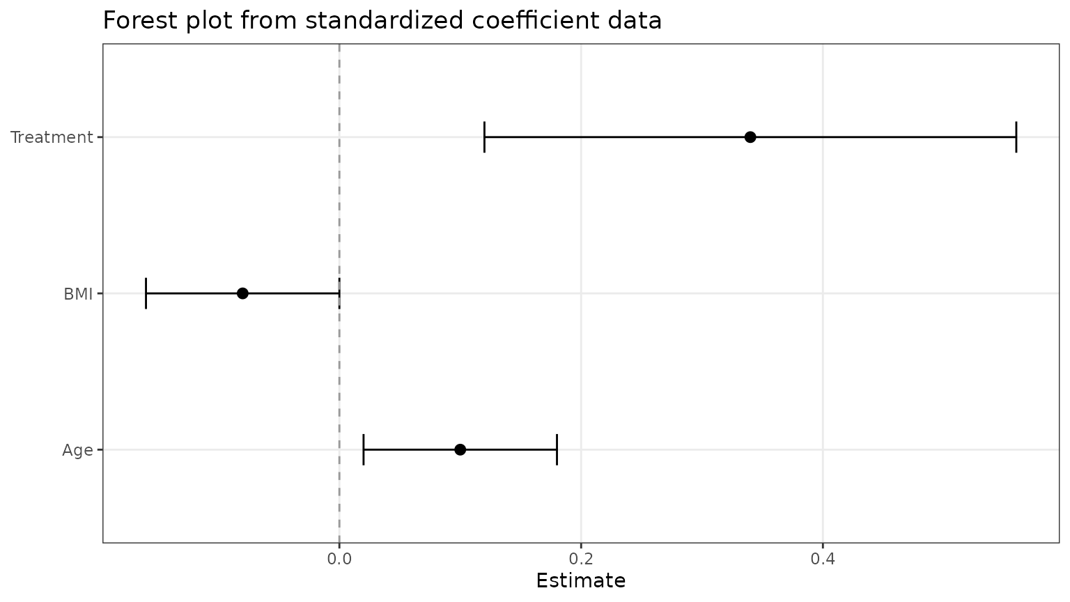
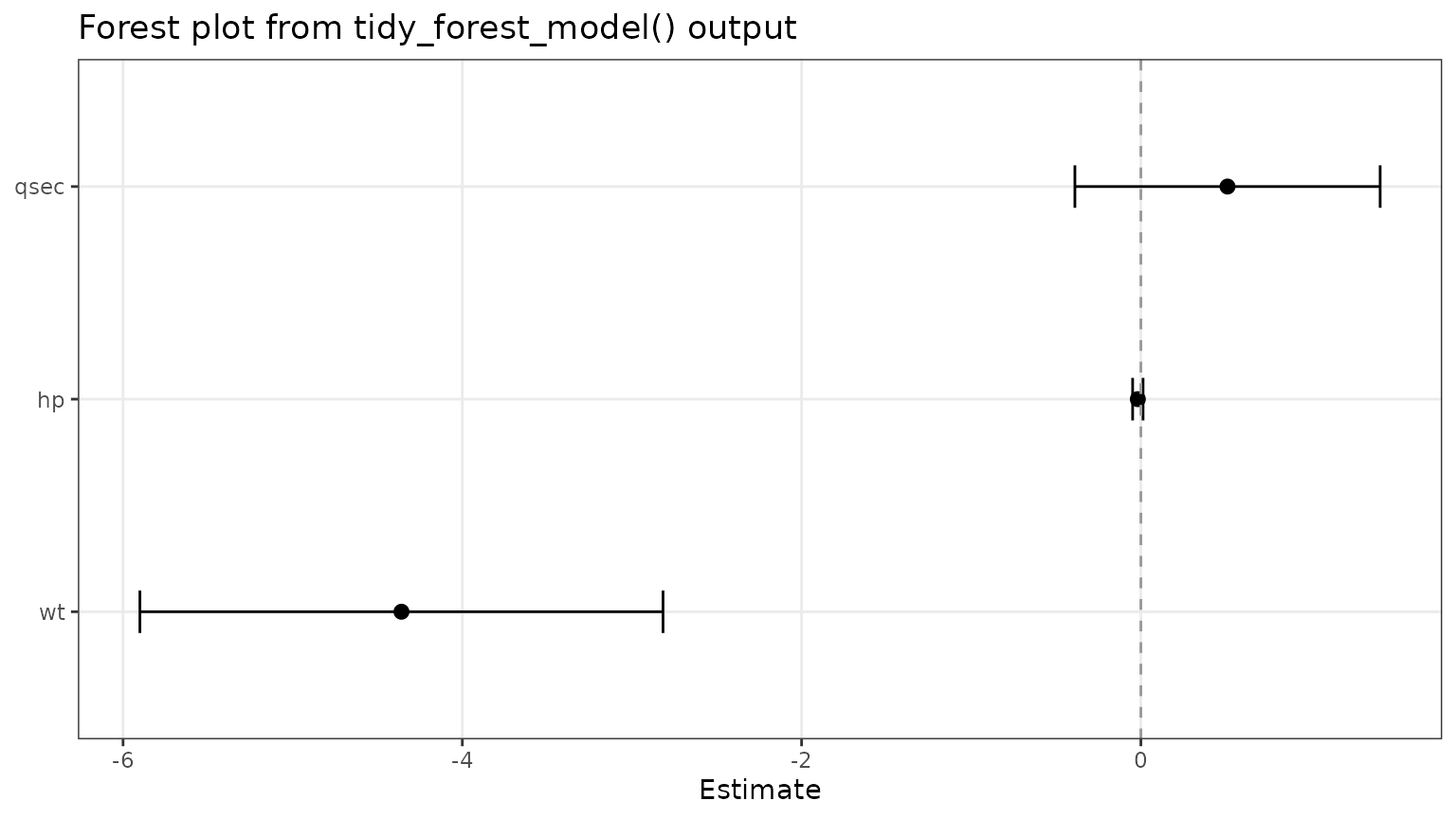
  ggplot2::labs(title = "Forest plot from standardized coefficient data")

Use tidy_forest_model() for model objects

If broom is available, tidy_forest_model() can pull coefficient estimates and confidence limits from a fitted model.

fit <- lm(mpg ~ wt + hp + qsec, data = mtcars)

model_ready <- tidy_forest_model(fit)

The returned object can be passed directly into ggforestplot().

ggforestplot(model_ready) +
  ggplot2::labs(title = "Forest plot from tidy_forest_model() output")

For logistic regression, set exponentiate = TRUE to return odds ratios instead of log-odds coefficients.

set.seed(123)

logit_data <- data.frame(
  age = rnorm(250, mean = 62, sd = 8),
  bmi = rnorm(250, mean = 28, sd = 4),
  treatment = factor(rbinom(250, 1, 0.45), labels = c("Control", "Treatment"))
)

linpred <- -9 +
  0.09 * logit_data$age +
  0.11 * logit_data$bmi +
  0.9 * (logit_data$treatment == "Treatment")

logit_data$event <- rbinom(250, 1, plogis(linpred))

logit_fit <- glm(event ~ age + bmi + treatment, data = logit_data, family = binomial())
logit_ready <- tidy_forest_model(logit_fit, exponentiate = TRUE)

ggforestplot(logit_ready) +
  ggplot2::labs(
    title = "Forest plot from exponentiated logistic regression output",
    x = "Odds ratio"
  )