Get Started with ggforestplotR
Source:vignettes/ggforestplotR-get-started.Rmd
ggforestplotR-get-started.RmdggforestplotR is built for coefficient-driven forest
plots that stay inside a normal ggplot2 workflow.
Choose a workflow
Use the package in one of two ways:
- Start from a coefficient table and map the required columns directly to the plot.
- Start from a fitted model and let
tidy_forest_model()orggforestplot()callbroom::tidy()and create the plot.
This article covers some basic examples and the minimum data you need.
Start from a coefficient table
The simplest input is a data frame with a column for terms, estimates, and confidence limits. If your columns use different names, you can map them explicitly.
There is also functionality to rename term labels and sort terms to your liking, among other things.
basic_coefs <- data.frame(
  term = c("Age", "BMI", "Treatment"),
  estimate = c(0.10, -0.08, 0.34),
  conf.low = c(0.02, -0.16, 0.12),
  conf.high = c(0.18, 0.00, 0.56)
)

ggforestplot(basic_coefs,
             term_labels = c("Age" = "age", "BMI" = "bmi", "Treatment" = "trt"),
             sort_terms = "descending")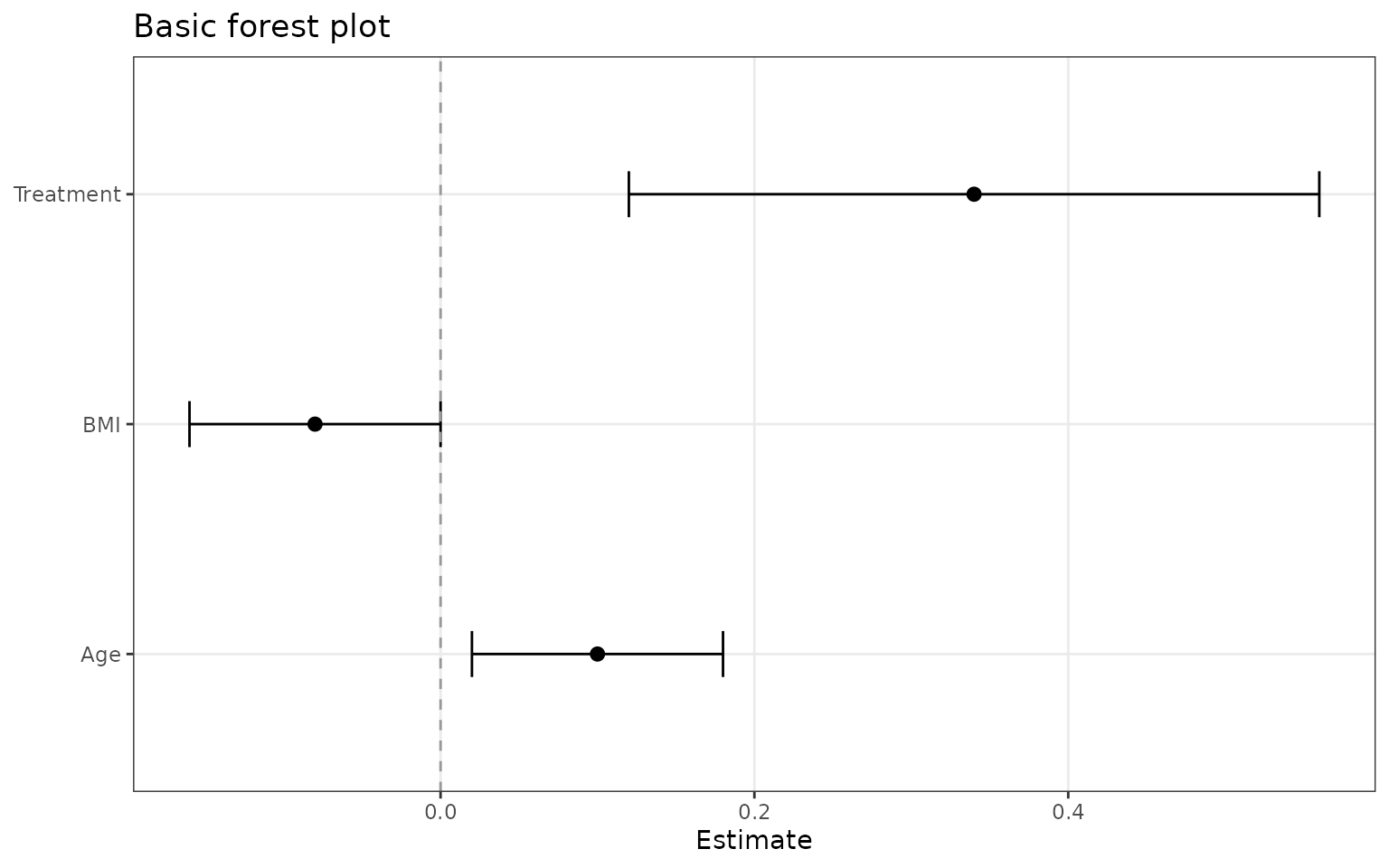
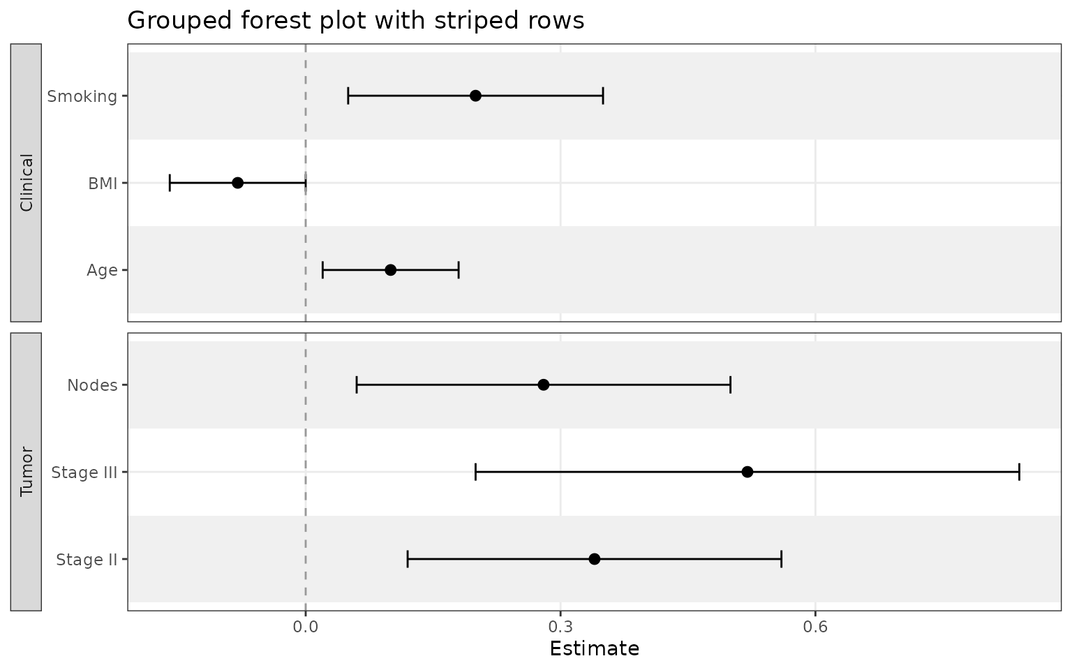
Add grouped sections and row striping
Use facet when you want related variables separated into
labeled panels. Add striped_rows = TRUE to color
alternating rows in the plot.
sectioned_coefs <- data.frame(
  term = c("Age", "BMI", "Smoking", "Stage II", "Stage III", "Nodes"),
  estimate = c(0.10, -0.08, 0.20, 0.34, 0.52, 0.28),
  conf.low = c(0.02, -0.16, 0.05, 0.12, 0.20, 0.06),
  conf.high = c(0.18, 0.00, 0.35, 0.56, 0.84, 0.50),
  section = c("Clinical", "Clinical", "Clinical", "Tumor", "Tumor", "Tumor")
)

ggforestplot(
  sectioned_coefs,
  facet = "section",
  striped_rows = TRUE,
  stripe_fill = "grey94",
  facet_strip_position = "right",
  sort_terms = "ascending"
)
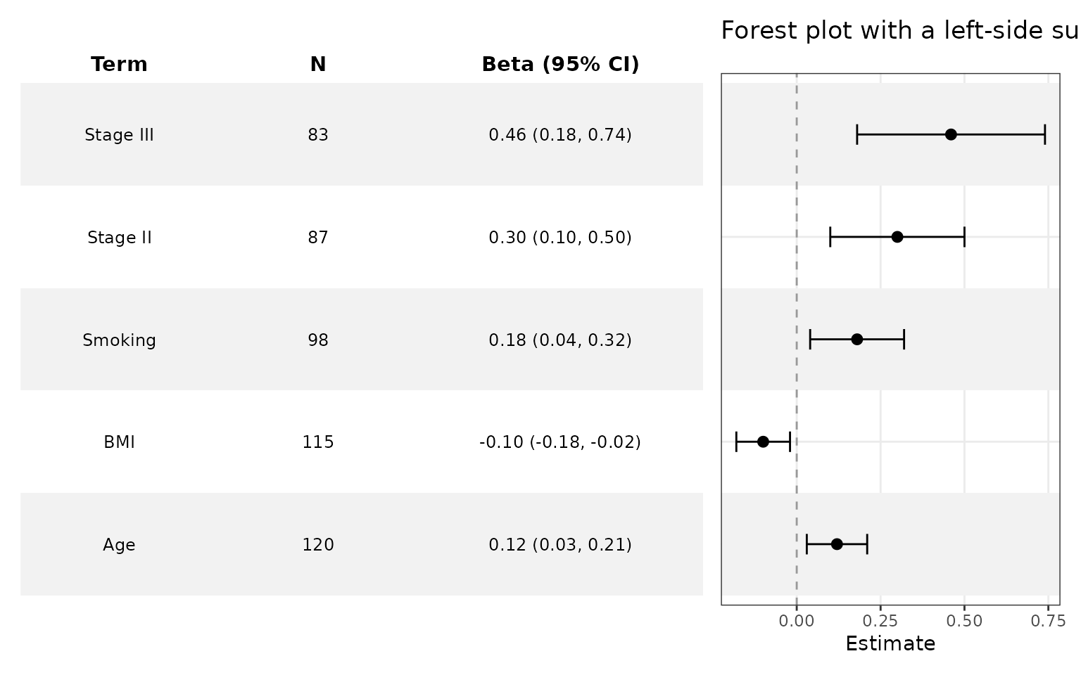
Add a summary table
Use add_forest_table() to add a summary table to your
forest plot.
tabled_coefs <- data.frame(
  term = c("Age", "BMI", "Smoking", "Stage II", "Stage III"),
  estimate = c(0.12, -0.10, 0.18, 0.30, 0.46),
  conf.low = c(0.03, -0.18, 0.04, 0.10, 0.18),
  conf.high = c(0.21, -0.02, 0.32, 0.50, 0.74),
  sample_size = c(120, 115, 98, 87, 83)
)

ggforestplot(tabled_coefs, striped_rows = TRUE) +
  add_forest_table(
    position = "left",
    column_labels = c("term" = "Variable", "sample_size" = "N", "estimate" = "Beta (95% CI)"),
    columns = c("term", "sample_size", "estimate"),
    estimate_digits = 2,
    interval_digits = 3
  )
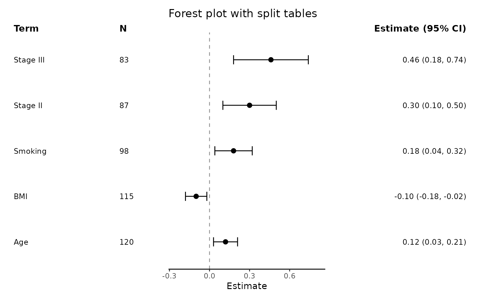
Add split summary tables
Use add_split_table() to create a more traditional
looking forest plot, with summary data on either side of the plot.
ggforestplot(tabled_coefs, n = "sample_size", striped_rows = T) +
  add_split_table(
    left_columns = c("term", "n"),
    right_columns = c("estimate"),
    column_labels = c("term" = "Variable", "estimate" = "Beta (95% CI)")
  )
Start from a fitted model
If broom is installed, ggforestplot() can
work directly from a fitted model.
fit <- lm(mpg ~ wt + hp + qsec, data = mtcars)

ggforestplot(fit, sort_terms = "descending",
             term_labels = c("wt" = "Weight"),
             striped_rows = T) +
  scale_x_continuous(breaks = seq(-6,2,1)) +
  add_forest_table()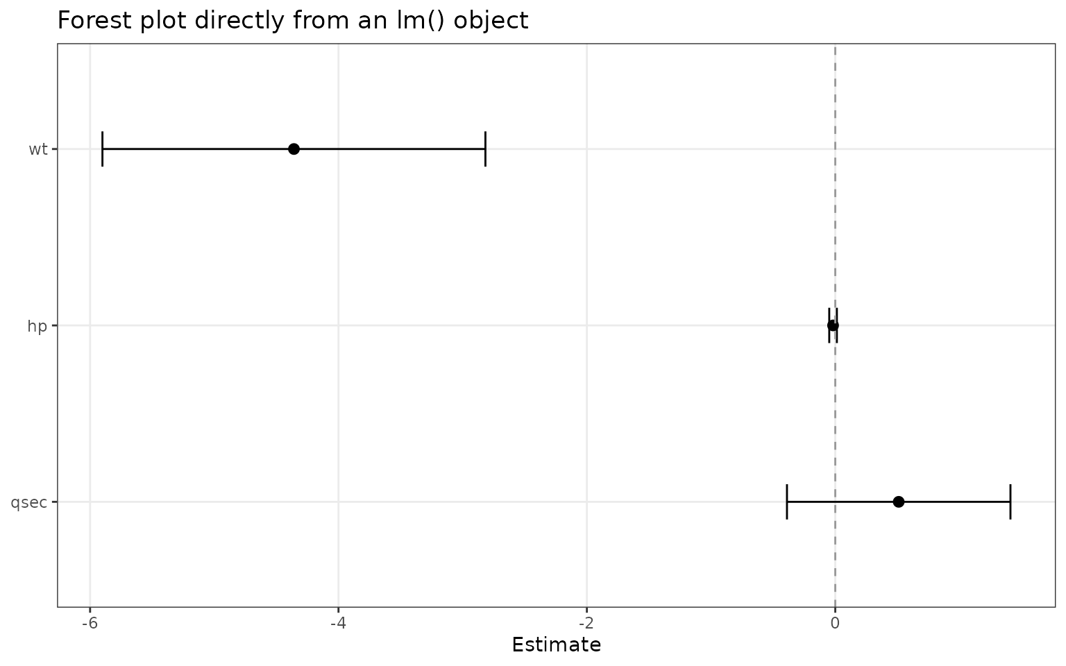
Next articles
For more detail, see:
-
ggforestplotR-plot-customizationfor enhanced customization of the plots and summary tables. -
ggforestplotR-data-helpersforas_forest_data()andtidy_forest_model().